
The convolution Engine

Now you can access an FPGA LAB environment on demand with chiprentals. This service is currently in the Beta stage and is being provided for free. Go perform your projects in a real world environment. Book your slot here. The PYNQ-Z2 board being offered currently is the best choice for trying out ML and AI acceleration projects like this one.
Part One - The Architecture Outline
Part Two - The Convolution Engine
Part Three - The Activation Function
Part Five - Adding fixed-point arithmetic to our design
Part Six - Generating data and automating the Verification Process
Part Seven - Creating a multi-layer neural network in hardware.
- From here on we shall refer to a convolution layer as a
convlayer. - Our design implements a fully parameterized convolution operation in Verilog. By 'fully parameterized', I mean to say that the same code can be used to synthesize a
convlayer of any size the architecture demands(conv3x3,conv7x7,conv11x11). You just have to vary the parameters passed to this code before the synthesis. - The primary idea behind the approach to this design is to build a highly pipelined streaming architecture wherein the processing module does not have to stop at any point in time. i.e any part of the convolver does not wait for any other part to finish its work and supply it with the result. Each stage is performing a small portion of the entire work continuously on a different part of the input every clock cycle. This is not just a feature of this design, it is a general principle called 'pipelining' that is widely used to break down large computational processes into smaller steps and also increase the highest frequency that the entire circuit can operate at.
- Our design uses the MAC (Multiply and Accumulate) units with the aim of mapping these operations to the DSP blocks of the FPGA. Achieving that would make the multiplication and addition operations much faster and consume less power since the DSP blocks are implemented in hard macros. which is to say, the DSP blocks have already been synthesized, placed, and routed into silicon on the FPGA device in the most efficient way possible, unlike general IP blocks wherein only the tried and tested RTL code is supplied to you and can be synthesized at your will.
- The convolver is nothing but a set of MAC units and a few shift registers, which when supplied with the right inputs, output the result of the convolution after a fixed number of clock cycles. Let's Dig into it!
- Let us assume the size of the input Feature map (image) to be of a dimension
NxNand our kernel (filter/window) to be of the dimensionsKxK. It is understood obviously, thatK < N. -
srepresents the value of the stride with which the window moves over the feature map.Now, if you know how the 2-D convolution works, the size of the output feature map will be smaller than that of the input feature map. Precisely, if we do not have some form of zero paddings on the input feature map, the output will be of the size
(N-K+1)/s x (N-K+1)/sAs you can see in the image, our convolver has MAC units laid out in the size of the convolution kernel and a couple of shift registers connected at various levels in the pipeline. The thing to note about the inputs to these various MAC units is that.
- The kernel weights are placed such that each MAC unit has a fixed value of the weight throughout the process of the convolution, but each mac unit has a different value placed on it according to its position.
- Whereas, for the input activation values, the same value is placed on each and every one of the MAC units except that value changes with every clock cycle according to the input feature map.
Additionally, we have a few more signals like the
valid_convandend_convsignal which tell the outside world if the outputs of this convolver module are valid or not. But why would the convolver produce invalid results in the first place? After the window is done moving over a particular row of the input, it continues to wrap around to the next row creating invalid outputs. We could avoid calculation during the wrap-around period, but that would require us to stop the pipeline, which is against our streaming design principle. So instead we just discard the outputs that we believe are invalid with the help of avalid convsignal. Look at the following animation to understand better.
This animation shows how the various inputs to the Convolver are being modified with each clock cycle and also tracks the value of a particular variable as it makes its way to the output, this shows you the mathematical reasoning behind the design and how the convolution is actually being calculated.
If you observe the final value of
xwhich isw0*a0 + w1*a1 + w2*a2 + w3*a4 + w4*a5 + w5*a6 + w6*a8 + w7*a9 + w8*a10The code snippet pertaining to the convolution unit has been shown below. It is fairly well commented and uses the Verilog generate loop to simplify the code for all those MAC units, also, the code is fully parameterized, meaning you can scale it to any size of
NandKyou wish depending on which neural network you are building.ADVANTAGES OF THIS ARCHITECTURE:
- The input feature map has to be sent in only once (i.e the stored activations have to be accessed from the memory only once) thus greatly reducing the memory access time and the storage requirement. The shift registers create a kind of local caching for the previously accessed values.
- The convolution for any sized input can be calculated with this architecture without having to break the input or temporarily store it elsewhere due to low compute capability
- The stride value can also be changed for some exotic architectures where a larger stride is required.
Now let's dig into:
The Code
Before we start writing Verilog for our design, we need to have a golden model. i.e. a basic model in code that is able to achieve the functionality we are targeting to create in hardware. You can code it in which ever language you like, but I choose python because I love python.
import numpy as np
from scipy import signal

ksize = 3      															#ksize x ksize convolution kernel
im_size = 4   															#im_size x im_size input activation map

def strideConv(arr, arr2, s): 											  #the function that performs the 2D convolution
    return signal.convolve2d(arr, arr2[::-1, ::-1], mode='valid')[::s, ::s]

kernel =  np.arange(0,ksize*ksize,1).reshape((ksize,ksize))                   #the kernel is a matrix of increasing numbers
act_map = np.arange(0,im_size*im_size,1).reshape((im_size,im_size))           #the activation map is a matrix of increasin numbers

conv = strideConv(act_map,kernel,1)
print(kernel)
print(act_map)
print(conv)
Running the above code gives us:
kernel
 [[0 1 2]
 [3 4 5]
 [6 7 8]]

activation map
 [[ 0  1  2  3]
 [ 4  5  6  7]
 [ 8  9 10 11]
 [12 13 14 15]]

convolution output
 [[258 294]
 [402 438]]
So our goal would be to design a Verilog module that achieves the same set of outputs for any given inputs to the above python function.
NOTE on utilizing DSP blocks for MAC units - when the synthesis tools encounter a multiply and accumulate operation, they usually implement that code in a
DSP block on the FPGA instead of using regular slice logic. However in some cases like high resource utilization scenarios the tools do not have enough dsp
blocks and implement multipliers and adders in regular slice logic instead. To be sure, we could use the (* use_dsp = "yes" *) attribute in xilinx or a
similar attribute in other tools (extract_mac for Altera tools) to force them to use the relevant DSP resources on the FPGA for that particular module.However, it is not necessary in
most cases.
This document from Xilinx and this one from intel will tell you more about this stuff.
I have written lots of comments in the code to better explain it -
//file: convolver.v
`timescale 1ns / 1ps

module convolver #(
parameter n = 9'h00a,     // activation map size
parameter k = 9'h003,     // kernel size
parameter s = 1,          // value of stride (horizontal and vertical stride are equal)
parameter N = 16,         //total bit width
parameter Q = 12          //number of fractional bits in case of fixed point representation.
)(
input clk,
input ce,
input global_rst,
input [N-1:0] activation,
input [(k*k)*16-1:0] weight1,
output[N-1:0] conv_op,
output valid_conv,
output end_conv
);

reg [31:0] count,count2,count3,row_count;
reg en1,en2,en3;

wire [15:0] tmp [k*k+1:0];
wire [15:0] weight [0:k*k-1];

//breaking our weights into separate variables. We are forced to do this because verilog does not allow us to pass multi-dimensional
//arrays as parameters
//----------------------------------------------------------------------------------------------------------------------------------
generate
	genvar l;
	for(l=0;l<k*k;l=l+1)
	begin
        assign weight [l][N-1:0] = weight1[N*l +: N];
	end
endgenerate
//----------------------------------------------------------------------------------------------------------------------------------
assign tmp[0] = 32'h0000000;

//The following generate loop enables us to lay out any number of MAC units specified during the synthesis, without having to commit to a //fixed size
generate
genvar i;
  for(i = 0;i<k*k;i=i+1)
  begin: MAC
    if((i+1)%k ==0)                       //end of the row
    begin
      if(i==k*k-1)                        //end of convolver
      begin
      (* use_dsp = "yes" *)               //this line is optional depending on tool behaviour
      mac_manual #(.N(N),.Q(Q)) mac(      //implements a*b+c
        .clk(clk),                        // input clk
        .ce(ce),                          // input ce
        .sclr(global_rst),                // input sclr
        .a(activation),                   // activation input [15 : 0] a
        .b(weight[i]),                    // weight input [15 : 0] b
        .c(tmp[i]),                       // previous mac sum input [32 : 0] c
        .p(conv_op)                       // output [32 : 0] p
        );
      end
      else
      begin
      wire [N-1:0] tmp2;
      //make a mac unit
      (* use_dsp = "yes" *)               //this line is optional depending on tool behaviour
      mac_manual #(.N(N),.Q(Q)) mac(
        .clk(clk),
        .ce(ce),
        .sclr(global_rst),
        .a(activation),
        .b(weight[i]),
        .c(tmp[i]),
        .p(tmp2)
        );

      variable_shift_reg #(.WIDTH(32),.SIZE(n-k)) SR (
          .d(tmp2),                  // input [32 : 0] d
          .clk(clk),                 // input clk
          .ce(ce),                   // input ce
          .rst(global_rst),          // input rst
          .out(tmp[i+1])             // output [32 : 0] q
          );
      end
    end
    else
    begin
    (* use_dsp = "yes" *)               //this line is optional depending on tool behaviour
   mac_manual #(.N(N),.Q(Q)) mac2(
      .clk(clk),
      .ce(ce),
      .sclr(global_rst),
      .a(activation),
      .b(weight[i]),
      .c(tmp[i]),
      .p(tmp[i+1])
      );
    end
  end
endgenerate

//The following logic generates the 'valid_conv' and 'end_conv' output signals that tell us if the output is valid.
always@(posedge clk)
begin
  if(global_rst)
  begin
    count <=0;                      //master counter: counts the clock cycles
    count2<=0;                      //counts the valid convolution outputs
    count3<=0;                      // counts the number of invalid onvolutions where the kernel wraps around the next row of inputs.
    row_count <= 0;                 //counts the number of rows of the output.
    en1<=0;
    en2<=1;
    en3<=0;
  end
  else if(ce)
  begin
    if(count == (k-1)*n+k-1)        // time taken for the pipeline to fill up is (k-1)*n+k-1
    begin
      en1 <= 1'b1;
      count <= count+1'b1;
    end
    else
    begin
      count<= count+1'b1;
    end
  end
  if(en1 && en2)
  begin
    if(count2 == n-k)
    begin
      count2 <= 0;
      en2 <= 0 ;
      row_count <= row_count + 1'b1;
    end
    else
    begin
      count2 <= count2 + 1'b1;
    end
  end

  if(~en2)
  begin
  if(count3 == k-2)
  begin
    count3<=0;
    en2 <= 1'b1;
  end
  else
    count3 <= count3 + 1'b1;
  end
  //one in every 's' convolutions becomes valid, also some exceptional cases handled for high when count2 = 0
  if((((count2 + 1) % s == 0) && (row_count % s == 0))||(count3 == k-2)&&(row_count % s == 0)||(count == (k-1)*n+k-1))
  begin
    en3 <= 1;
  end
  else
    en3 <= 0;
end
	assign end_conv = (count>= n*n+2) ? 1'b1 : 1'b0;
	assign valid_conv = (en1&&en2&&en3);
endmodule
As you can notice in the above code, we use the MAC units and shift registers to lay out the planned architecture. While the shift register is a straight forward shift-register module wherein you can supply the data width and depth of the shift register as parameters, the mac_manual module is also quite simple to implement, at least when we are working with integers.
//file: mac_manual.v
//note that this file has been modified after the addiion of fixed point arithmetic support
//this post has not been edited for the same keeping in mind first time readers. Do refer
//to that post in this series.

module mac_manual #(
	parameter N = 16,
    parameter Q = 12
    )(
    input clk,sclr,ce,
    input [N-1:0] a,
    input [N-1:0] b,
    input [N-1:0] c,
    output reg [N-1:0] p
    );

always@(posedge clk,posedge sclr)
 begin
    if(sclr)
    begin
        p<=0;
    end
    else if(ce)
    begin
        p <= (a*b+c);                   //performs the multiply accumulate operation
    end
 end
endmodule
Verifying our design with a testbench
//convolver_tb.v

`timescale 1ns / 1ps
module convolver_tb;

	// Inputs
	reg clk;
	reg ce;
	reg [143:0] weight1;
	reg global_rst;
	reg [15:0] activation;

	// Outputs
	wire [31:0] conv_op;
	wire end_conv;
	wire valid_conv;
	integer i;
    parameter clkp = 40;
	// Instantiate the Unit Under Test (UUT)
	convolver #(9'h004,9'h003,1) uut (
		.clk(clk),
		.ce(ce),
		.weight1(weight1),
		.global_rst(global_rst),
		.activation(activation),
		.conv_op(conv_op),
		.end_conv(end_conv),
		.valid_conv(valid_conv)
	);

	initial begin
		// Initialize Inputs
		clk = 0;
		ce = 0;
		weight1 = 0;
		global_rst = 0;
		activation = 0;
		// Wait 100 ns for global reset to finish
		#100;
         clk = 0;
		ce = 0;
		weight1 = 0;
		activation = 0;
         global_rst =1;
         #50;
         global_rst =0;
         #10;
		ce=1;
        //we use the same set of weights and activations as the sample input in the golden model (python code) above.
		weight1 = 144'h0008_0007_0006_0005_0004_0003_0002_0001_0000;
		for(i=0;i<255;i=i+1) begin
		activation = i;
		#clkp;
		end
	end
      always #(clkp/2) clk=~clk;
endmodule
Running the above test bench gives us the following result in Vivado:
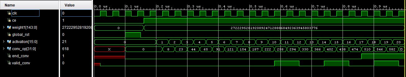
The values corresponding to the state when the valid_conv signal is high are the convolution outputs. Its quite clear that these outputs match the ones the python script gave us for the same input.
Here is a link to the exact git commit at this point. i.e before adding the Fixed-point arithmetic support to this project.
Fixed-point Arithmetic
You might wanna read this post, further in this series and come back to understand the changes we're about to make.
The advantage of a fully modular device like ours is that we only have to change the arithmetic (addition and multiplication) modules in order to get the whole thing working with fixed point numbers. Nothing else needs to be changed as the concept of that binary point is only in our heads. The hardware still only sees regular integers (bit-fields).
//file: mac_manual_fp
module mac_manual_fp(
    input clk,sclr,ce,
    input [15:0] a,
    input [15:0] b,
    input [31:0] c,
    output reg [31:0] p
    );
    wire [31:0] sum;
    wire [31:0] m;

qmult #(3,12) mul(a,b,m);            //The fixed-point multiplier module
qadd  #(3,12) add(m,c,sum);          //The fixed-point adder module
always@(posedge clk,posedge sclr)
 begin
    if(sclr)
    begin
        p<=0;
    end
    else if(ce)
    begin
        p <= sum;
        //p <= (a*b+c);               //The previous mac_manual operation for regular integers
    end
 end
endmodule
We just need to change the convolver.v module to call macmanualfp instead of mac_manual. To understand how the qmult and qadd arithmetic modules work, you might wanna go through this post and come back.
All the design files along with their test benches can be found at the Github Repo
PREVIOUS:The architecture outline
NEXT :The activation function